Correlation for Time Delay Analysis

Time delay analysis finds the delay (also called the “lag”) between two signals, that are shifted in time. It is the most important part of time-difference-of-arrival (TDOA) transmitter localization. This article presents an introduction to time delay analysis with application to TDOA localization with RTL-SDRs.

For delay analysis, correlation in the time domain is widely used. The correlation function plots the similarity between two signals for all possible lags \tau.

Corr(\tau) = \sum_{t=0}^{N-1}s_1(t)s_2(t+\tau)

The peak of the correlation function occurs at the lag with the best similarity between the two signals, i.e. the estimated delay.

\tau_{estimated} = \underset{\tau}{\arg\max} (Corr(\tau))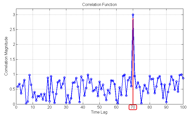

For robust determination of the delay, it is important to be able to read out the peak of the correlation function precisely. For that purpose, the correlation should have a distinct and outstanding peak (“good quality”). If, on the other hand, many peak are potential lags or a peak is distributed among several bins, accurate measurement of delay becomes difficult (“bad quality”).

The quality of the correlation is influenced by different parameters:

• The type of received RF signal (especially its bandwidth)
• The different properties of the receivers
• The different propagation paths between transmitter and the receivers
• The applied correlation method

Which signals exhibit good correlation properties?

The quality of correlation is first of all largely dependent on the transmitted signal. If the designer has the freedom to choose the transmitted signal, he should use one with known good correlation properties such as a Barker code or maximum-length-sequences. In generic TDOA systems the designer has no influence on the transmitted signal. In either case it is useful to understand the influence of the signal type on correlation.

In general there is a strong connection between bandwidth and correlation quality. Signals with large bandwidth and noise-like waveforms (e.g. maximum-length-sequences) correlate much better than narrow-band signals, that exhibit strong periodicity, as depicted below.

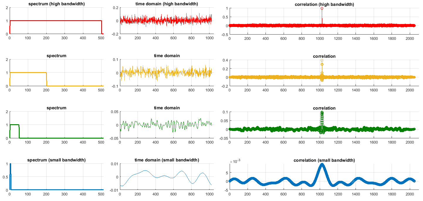
In theory, the correspondence between correlation and bandwidth is established by the Wiener-Khinchin-Theorem. In essence, it says that the power spectrum of a signal equals the power spectrum of its autocorrelation function (autocorrelation = correlation of a signal with a time-delayed version of itself). The perfect (and desirable) correlation is a single sharp peak. The power spectrum of such a sharp peak is wideband and following the theorem, so is the power spectrum of the time signal.

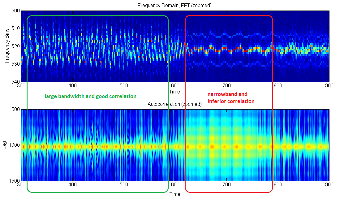
It needs to be emphasized, that bandwidth here refers to the “short-time” bandwidth of the signal  portion located in the correlation window and not the “general” bandwidth over a very long time. This is because only a comparatively short slice (or window) of the RF signal stream can be used for time delay analysis. Example:  A FM signal may have a bandwidth of several 10 kHz in general (over a long period). The window used for correlation is 10,000 samples. Then the “short-time” bandwidth in this short window needs to be considered. The short-time bandwidth of a FM signal, however, is strongly dependent on the transmitted content (silence corresponds to a sine wave and thus a very narrow bandwidth).

The figure below shows the bandwidth and correlation of successive slices of an FM signal. Bandwidth and correlation largely vary. It is advantageous to analyze the received signals and perform correlation on those slices, that have large bandwidth only.

Time delay analysis for complex IQ signals

Most radios, such as the RTL-SDR, deliver IQ samples at its output that can be interpreted as a complex signal, exhibiting a phase and amplitude information. In the following, s_1(t) is the complex IQ signal from one receiver and s_2(t) the complex IQ signal from the other receiver. Again the time delay between the signals is to be found using the correlation function.

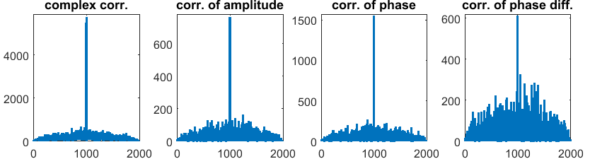
For IQ signals, four different variants of the correlation function are considered here:

1. Complex correlation is the standard approach to calculate the correlation of complex signals: |\sum s_1(t) \cdot s_2^*(t+\tau)| with * denoting “complex conjugate”.
2. Real-valued correlation of the amplitude, or the absolute value (magnitude), of the signals  \sum |s_1(t)| \cdot |s_2(t+\tau)|
3. Real-valued correlation of the phase of the signals \sum \measuredangle s_1(t) \cdot \measuredangle s_2(t+\tau) with \measuredangle s = \arg(s)
4. Real-valued correlation of the phase difference of the signals \sum [ \measuredangle s_1(t) - \measuredangle s_1(t-1)] \cdot [ \measuredangle s_2(t+\tau) - \measuredangle s_2(t-1+\tau)]

For any correlation method it is advantageous to remove the DC component of the input signals. (It mitigates the effect that the correlation function tends to have larger values at the center)

The applicability of the different methods is dependent on the modulation of the signal. The correlations based on phase and phase difference only respond to angular modulation (most used modulation types exhibit some component of angular modulation). Correlation of amplitude responds to amplitude modulation only, i.e. they hardly work on constant envelope modulation, such as FM. The method of complex correlation takes into account both amplitude and phase and is therefore suited for all modulation types.

However, modulation type is not the only criterion for choosing a specific correlation method. It is also dependent on different real-world flaws that will be considered below.

The influence of phase, amplitude and frequency offset

In a TDOA system, two receivers ideally output two identical versions of the signal, having only a time-shift between them. In real-world systems, both signals also differ in other parameters, like amplitude, phase and frequency offset.

A constant amplitude offset may originate in different propagation paths or receiver gain settings. Fortunately, it does not impact time delay analysis.

Differences in phase and frequency may originate in separate receivers, when phase and frequency of local oscillators and sampling circuits are not exactly synchronized (which is difficult in when the receivers are not located in the same place). Especially the use of low-cost radios like the RTL-SDR practically limits synchronization capabilities. While usually a constant phase offset does impact time delay analysis, frequency offsets are of greater interest, because they influence the results of correlations using phase information.

Frequency Offset:  For the analysis of frequency offset, a signal has been captured by an RTL-SDR sampling at 2 Msps. Then the correlation of this signal with a frequency shifted version of itself is analyzed to model a frequency offset in the receiver.

The influence of the frequency offset is strongly dependent on the used correlation method and the window size. The figures below show the four different correlations under frequency offset for a window size of 1,000,000 and 10,000 samples.

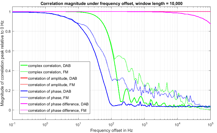
For a window size of 1,000,000 samples even tiny frequency offsets above some Hz make the complex correlation and correlation of phase useless. For shorter windows the tolerance on frequency offsets is greater. But even then frequency offsets need to be kept below some 100 Hz.

The simulations also show that the correlation of the amplitude and the correlation of the phase difference are robust against frequency offsets. The correlation of phase differences works well up to some 100 kHz. The correlation of amplitude values shows no impact at all, because it does not use phase information.

Robustness to noise

In general, all correlation methods are very robust to noise, if the noise components in the two signals are independent to some extent (This is because two perfectly independent noise signals do not correlate at all). In practical systems, noise is not always completely independent and the correlation methods exhibit different robustness to noise. The figure above shows, that correlation of the phase difference is slightly less robust to noise than the other three correlation methods. This is supported by the general observation that the differentiation operation amplifies noise. This should be considered when dealing with very low SNRs.

How to choose the window size?

The length of the window used for correlation analysis is a trade-off between several goals. The window length should be

1. large enough to provide a sufficient signal overlap, if the receivers cannot be triggered in time accurately
2. large enough to average signal differences others than time delay, such as noise and distortion originating in the different propagation path and physically different receivers
3. small enough to reduce the impact of frequency offset (unless correlation of the amplitude or the phase difference is used)
4. small enough to reduce the amount of required calculations and amount of data to be exchanged between the receivers

Comment on  1: A pair of internet connected RTL-SDR receivers can be simultaneously triggered with an accuracy of approximately some hundred milliseconds using SSH commands. This requires the window length to be larger than this time delay in order to capture a signal portion, that overlaps. For a trigger accuracy of 200 ms and a sample rate of 2 Msps, the window length must be at least 400,000 samples.

Summary and Recommendations

Careful selection of the correlation method improves the robustness and avoids errors in time delay measurements for complex IQ signals.

Correlation Method	Considered Information	Robust to Noise	Robust to Frequency Offset	Applicability to modulation type	Overall
Complex	Amplitude & Phase	++	—	all	–
Amplitude	Amplitude only	++	++	Amplitude mod. only (no FM)	+
Phase	Phase only	++	—	Angle mod. only	– –
Phase difference	Phase only	+	+	Angle mod. only	+ +

In summary, complex correlation should be chosen, whenever the receivers are exactly synchronized in frequency. If a frequency offset cannot be avoided, the correlation of amplitude or the correlation of the differential phase should be considered. Correlation of the phase is not recommended.

In a practical TDOA system based on RTL-SDRs the correlation of amplitude and/or phase difference may be suited most.

In any case, the modulation type of the analyzed signal should be considered, especially for constant envelope modulation (FM) correlation of amplitude is not applicable.

The achievable resolution and measurement accuracy is mostly dependent on the bandwidth and modulation of the received signal, which cannot be influenced by the receiver.