Time-frequency representations are used to analyze time-varying signals with respect to their spectral contents over time. Apart from the commonly used short-time Fourier transform, advanced methods can provide higher resolution. This article presents the wavelet transform, Wigner-Ville distribution and reassignment techniques for high-resolution time-frequency representation of RF signals.
Short-Time Fourier and Gabor Transform
The Short-Time Fourier transform (STFT) is the most widely known and commonly used time-frequency representation. It is well understood, easy to interpret and there exist fast implementations (FFT). Its drawbacks are the limited and fixed resolution in time and frequency.
The idea of the STFT is to move a sliding window w(t) over the signal x(t) to be analyzed, such that a particular time span of the signal is selected. For each position of the window a Fourier transform is calculated, that represents the frequency content of that time span. The STFT results in the two dimensional time-frequency representation:
X(t,f)=\intop_{-\infty}^{\infty}x(t_{1})w^{*}(t_{1}-t)e^{-j2\pi ft_{1}}dt_{1}For spectral analysis the squared magnitude of the STFT S_{x}(t,f)=\left|X(t,f)\right|^{2} is considered, which is called spectrogram.
Time and frequency resolution can be controlled by the window length:
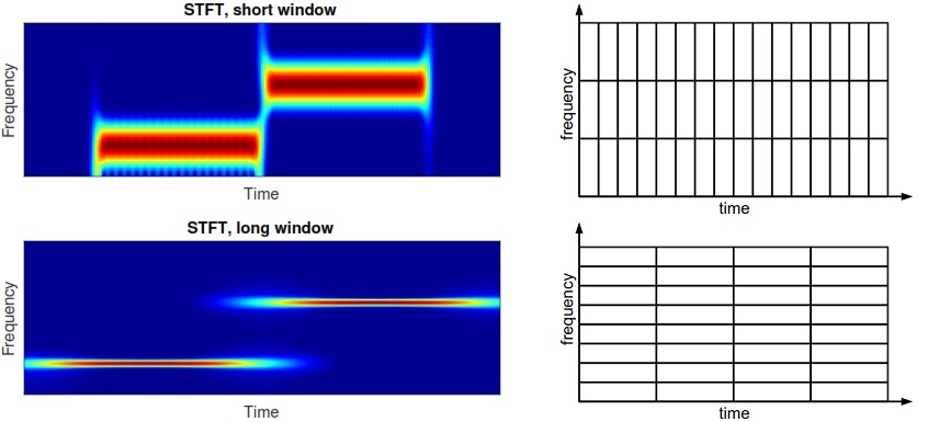
A short window captures only a short period of time and has thus a precise time resolution. However, the frequency resolution is poor, because the windowed signal contains only few time samples resulting in only few frequency bins during FFT calculation.
A long window provides poor time resolution, but creates precise frequency information due to the larger number of samples for the FFT.
Gabor transform
The trade-off between time and frequency resolution is known as the uncertainty principle. It states that the product of resolution in time and frequency is limited: BT \geq 1/4π (with B being the bandwidth of one frequency bin). A special case of the STFT is known as the Gabor transform. The Gabor transform fulfills the uncertainty equation above with equality, i.e. it has has the best joint time and frequency resolution. The Gabor transform is simply a STFT with the window being a Gaussian function w(t)=e^{-\alpha t^{2}}, where the parameter \alpha controls the window length, i.e. the emphasis on time or frequency resolution.
Wavelet Transform
The result of the wavelet transform differs from the STFT in that its time-frequency resolution is not fixed and depends on the frequency (multi-scale property, see Figure below). In general, the wavelet transform represents lower frequency components with finer frequency resolution and coarser time resolution. For higher frequencies the reverse is true: frequency resolution is coarser and time resolution is finer. This variable resolution property of the wavelet transform is sometimes superior to the Fourier approach, because it may give clearer spectral information for certain applications, such as audio signal processing.
The wavelet transform compares the time domain signal x(t) with a short analysis function \varPsi(t), analog to the STFT. \varPsi(t) is called the wavelet and can take on many forms as will be described below. During the calculation of the transform the wavelet is repeatedly moved over the signal (time shifted). In each pass the wavelet is scaled differently in time, i.e. dilated to a different length (dilation or scale). This creates a two dimensional representation of time (i.e. shift) and scale (can be related to frequency). The time shift is denoted by b, the scale by a. The continuous wavelet transform (CWT) is defined as:
CWT(a,b)=\frac{1}{\sqrt{a}}\intop_{-\infty}^{\infty}x(t)\varPsi^{*}\left(\frac{t-b}{a}\right)dtAnalog to the spectrogram of the STFT, the scalogram of the wavelet transform is defined as \left|CWT(a,b)\right|^{2} .
Different wavelet functions are available for analysis. For the CWT commonly Morlet wavelets (also called Gabor wavelets) are used, that consist of a complex sine wave with Gaussian envelope \varPsi_{Morlet}(t)=e^{-\alpha t^{2}}e^{j2\pi f_{c}t} . Here, the parameters fc (center frequency) and alpha (width of gaussian) control the trade-off between time and frequency resolution and need to be selected before conducting the transform. Basically, wavelet functions need to be functions that are both local in time and frequency to provide adequate time and frequency resolution. The Figure below shows an exemplary scalogram of a CWT.

Wigner-Ville Distribution (WVD)
The Wigner-Ville distribution (WVD) overcomes the limited resolution of the Fourier and wavelet based methods using an autocorrelation approach. The standard version of the autocorrelation function (ACF) considers the pointwise multiplication of a signal with a lagged version of itself and integrates the results over time. It is defined as
r_{xx}(\tau)=\intop_{-\infty}^{\infty}x(t)x^{*}(t+\tau)dt
The standard ACF is only dependent on the lag τ, because time is integrated out of the result. The WVD uses a variation of the ACF, called the instantaneous autocorrelation, which omits the integration step. Thus time remains in the result. The instantaneous autocorrelation is therefore a two dimensional function, depending on t and the lag τ
R_{xx}(t,\tau)=x(t+\frac{\tau}{2})x^{*}(t-\frac{\tau}{2})

As an example, the Figure above shows the instantaneous autocorrelation of a triangular shaped signal. The WVD calculates the frequency content for each time step t by taking a Fourier transform of the instantaneous autocorrelation across the axis of the lag variable τ for that given t:
\begin{align*}
W(t,f) & = \intop_{-\infty}^{\infty}R_{xx}(t,\tau)e^{-j2\pi f\tau}d\tau\\
 & = \intop_{-\infty}^{\infty}x(t+\frac{\tau}{2})x^{*}(t-\frac{\tau}{2})e^{-j2\pi f\tau}d\tau
\end{align*}
The result is real-valued. This way of calculation is related to the fact, that the Fourier spectrum of a signal equals the Fourier transform of its ACF. The WVD offers very high resolution in both time and frequency, that is much finer than the STFT.

An important disadvantage of the WVD are the so-called cross terms. These are ghost artifacts in the time-frequency representation (see Figure above). Cross-terms stem from the fact, that the WVD is a quadratic (and therefore a non-linear) transform. Cross terms extensively occur for all but very simple signals (sine, simple chirp). For most practical RF signals they spoil the result and thus limit the practical applicability of the WVD.
Smoothed Pseudo Wigner-Ville Distribution (SPWVD)
A method to reduce cross terms is to suppress them by additional low-pass filtering in time and frequency. This is possible because cross-terms typically have a fast oscillating behavior. However, this suppression of cross terms comes at the expense of reduced resolution.
Different shapes of these 2-dimensional low-pass filters (in time and frequency) can be applied and lead to different variants (Cohen’s class distributions). A prominent one is the smoothed pseudo Wigner-Ville distribution (SPWVD) . Other variants such as Choi-Williams, Margenau-Hill or Rihaczek can be found in literature, but often provide very similar results to the SPWVD for practical signals. The SPWVD is defined as the WVD filtered by two separate kernels g(t) and H(f) (need to be chosen prior to the transform), that smooth the WVD in frequency and time:
SPWVD(t,f)=\intop_{t_{1}}\intop_{f_{1}}g(t-t_{1})H(f-f_{1})W(t_{1,}f_{1})dt_{1}df_{1}The following figure shows the results of the smoothed pseudo Wigner-Ville distribution. The cross terms are suppressed at the cost of coarser resolution.

Reassignment
Reassignment is an effective way to “sharpen” a blurry spectrogram. The application of reassignment often leads to a time-frequency representation with very high resolution.
The calculations consist of two steps: spectrogram calculation (i.e. the short-time Fourier transform as described above), followed by the reassignment step. During reassignment every point (t, f) in the original spectrogram is moved to a new value (\hat{t}, \hat{f}) forming the reassigned spectrogram. For that purpose the phase of the short-time Fourier transform \Phi(t,f) is used, that is usually discarded when calculating the spectrogram only:
\hat{t}=t-\frac{1}{2\pi}\frac{\partial\Phi(t,f)}{\partial f}\hat{f}=\frac{1}{2\pi}\frac{\partial\Phi(t,f)}{\partial t}More details on the background of the reassignment technique can be found in the literature .

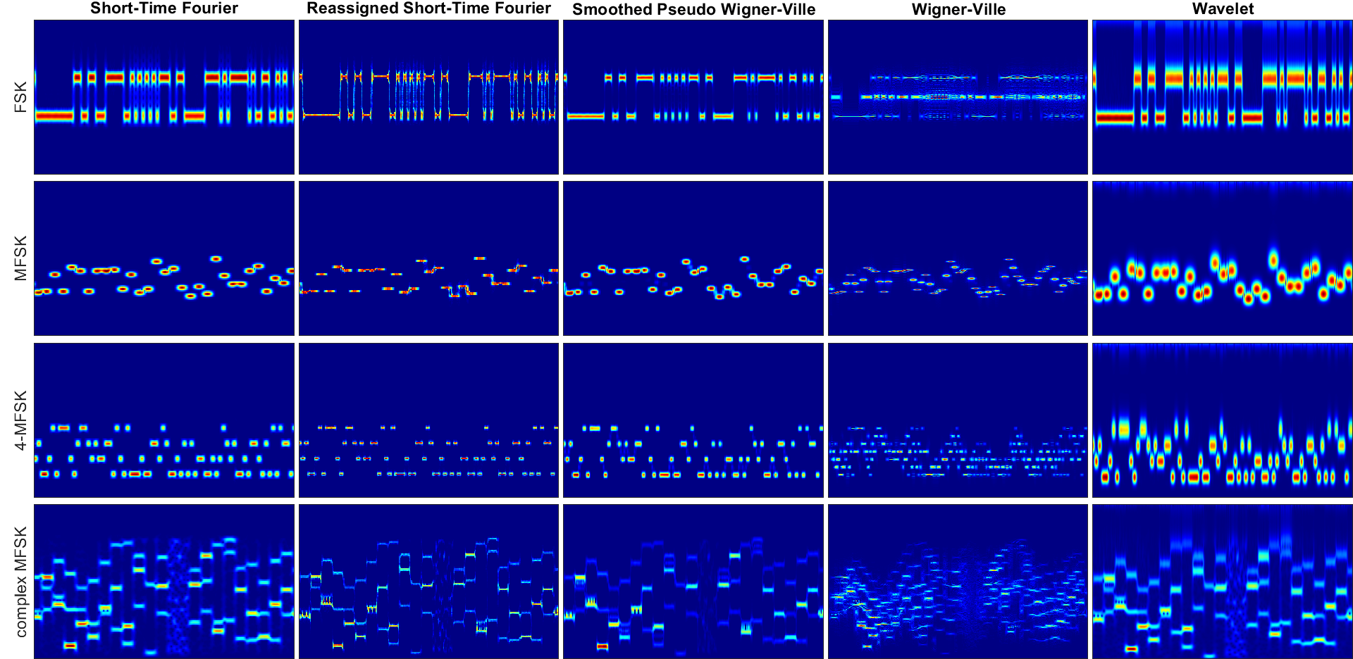
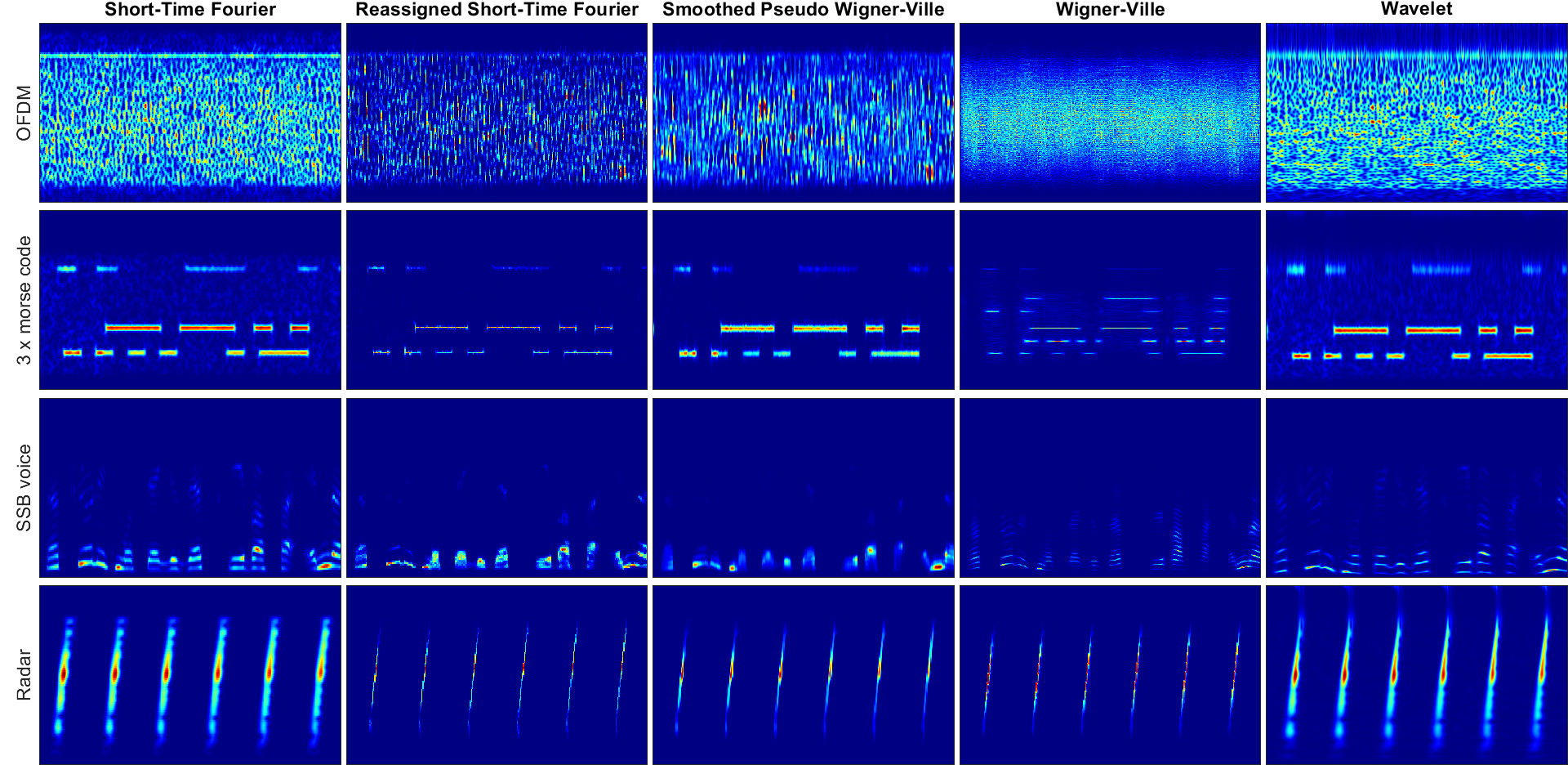
Examples of Time-Frequency Representations of Practical RF Signals
Conclusion
Although the Fourier transform is the standard algorithm for practical time-frequency analysis, other approaches can provide higher resolution. Especially time-frequency representations with reassignment techniques or the smoothed pseudo Wigner-Ville distribution have extremely fine resolution in both time and frequency, while having only little to no artifacts.
Further Reading
- My paper with an overview of time-frequency representations including many signal examples and some tips when to use which transform: Fourier, Gabor, Morlet or Wigner: Comparison of Time-Frequency Transforms
- Maria Sandsten’s (Lund University) extensive introduction: Time-Frequency Analysis of Time-Varying Signals and Non-Stationary Processes
- Another extensive introduction (IEEE Signal Processing Magazine): Linear and Quadratic Time-Frequency Signal Representations
- On reassignment: Flandrin et al., Time-Frequency reassignment: from principles to algorithms and Kodera et al., A new method for the numerical analysis of non-stationary signals


