This article investigates deep neural networks for wireless signal recognition or radio signal classification. It presents four different neural networks, that are able to classify IQ signals into 18 different wireless signal types. The networks are trained on a synthetically generated, but realistic, data set, considering a noisy HF channel environment under imperfect receiver conditions. The results of the best networks show an excellent validation accuracy of up to 98 % with reasonable training effort.
This article is a shortened version of my paper
Classification of Radio Signals and HF Transmission Modes with Deep Learning (2019)
Introduction to Wireless Signal Recognition
Wireless signal recognition is the task of determining the type of an unknown signal. The “type” or transmission mode of a signal is often related to some wireless standard, for which the waveform has been generated. Typical signal types depend on the frequency band of interest and could be Wi-Fi, 5G mobile, digital radio (DAB), radioteletype (RTTY), AM broadcasting or Morse code.
Recognition of radio signals is an essential task in signal intelligence and surveillance applications and is adopted in applications like cognitive radio and dynamic spectrum access to continuously monitor the spectrum and its occupancy by various different radio signals, modes and services.
Wireless signal recognition is a classification problem. Recently, advanced machine learning techniques, like deep neural networks, gained huge interest and showed extremely good performance for classification tasks in various applications. Instead of formulating hand-crafted features by a designer, a training algorithm uses large amounts of labelled example data to learn and extract good features from the data that are discriminative for the classification task.
This articles considers the recognition of 18 wireless radio signals typically present in the HF band (3-30 MHz) as a showcase example, because the HF band contains many different modes that coexist closely spaced in the frequency spectrum.
Data Set
The training dataset is the Panoradio HF dataset. The 18 wireless signal types (see Table below) cover very different modulation techniques, including analog (AM, facsimilie and SSB) and various digital modulation types (PSK, FSK, M-FSK, OOK, multicarrier). However, some types are very similar, such as RTTY45 and RTTY50, that differ only by their baud rate of 45 and 50 Bd and are expected to be especially hard to classify. Other similar types are PSK31 and PSK63, as well as SSB in upper (USB) and lower (LSB) sideband.
| Signal Type | Modulation | Baud Rate |
| Morse Code | OOK | variable |
| PSK31 | PSK | 31 |
| PSK63 | PSK | 63 |
| QPSK31 | QPSK | 31 |
| RTTY 45/170 | FSK, 170 Hz shift | 45 |
| RTTY 50/170 | FSK, 170 Hz shift | 50 |
| RTTY 100/850 | FSK, 850 Hz shift | 850 |
| Olivia 8/250 | 8-MFSK | 31 |
| Olivia 16/500 | 16-MFSK | 31 |
| Olivia 16/1000 | 16-MFSK | 62 |
| Olivia 32/1000 | 32-MFSK | 31 |
| DominoEx | 18-MFSK | 11 |
| MT63 | multi-carrier | 10 |
| Navtex / Sitor-B | FSK, 170 Hz shift | 100 |
| Single-Sideband (upper) | USB | – |
| Single-Sideband (lower) | LSB | – |
| AM broadcast | AM | – |
| HF/radiofax | radiofax | – |
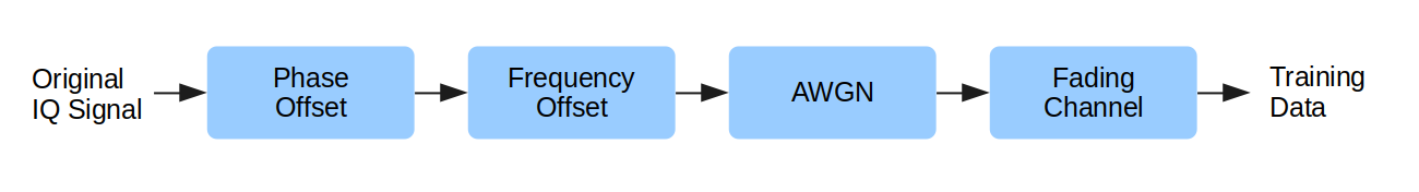
The training data is generated synthetically by simulation. First raw text, audio and images are modulated using standard software to generate a specific wireless signal type. Then the modulated signal is cut into short data signals. These signals are then artificially and randomly distorted according to a channel model. The model consists of random phase and frequency offsets, additive white Gaussian noise (AWGN) and a fading channel.
The fading channel follows the Watterson model, that introduces doppler shifts and frequency selective fading. The Watterson model is typically used to emulated ionospheric propagation as it occurs in HF communication. Furthermore, doppler shifts and frequency selective fading also occur in many other communication channels. For more information on the fading channel model, consider the original paper or the description of the Panoradio HF dataset.
Overall the following signal impairments are used:
- random frequency offset (+- 250 Hz)
- random phase offset
- AWGN noise (from -10 to +25 dB)
- Fading (CCIR 520 channel models “good”, “moderate”, “bad”, “flutter”, doppler”, no fading)
Transmission in the HF band is mostly characterized by comparably small bandwidths (often less than 3 kHz) and therefore low data rates. The data set contains vectors of complex IQ data of length 2048 with a sample rate of 6 kHz. Thus a data vector corresponds to a time of approximately 0.3 s. In total, the data set consists of 120,000 training vectors and another 30,000 vectors for validation.
Models and Training
This paper investigates four neural networks or models for wireless signal recognition, that range from ordinary convolutional neural nets to advanced models, like residual nets.
- Classical CNN: It consists of six convolutional layers each followed by max pooling. At the output two large dense layers are located.
- All Convolutional Net: It is only composed of convolutional layers with stride 2 (instead of max pooling layers) and it has a global average pooling layer at its output.
- Deep CNN: It uses 16 convolutional layers, with max pooling after every second convolutional layer and a single small dense layer at the output, roughly following the concept of the VGG net.
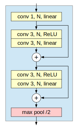
- Residual Net: It uses a large number of layers enhanced by residual connections. While the original residual net (He et al, 2015) did not provide convincing results, an arrangement of eight 5-layer residual stacks (O’Shea et al. 2017) proved to be more appropriate for the task of signal classification and is applied here.

The nets have a similar number of parameters around 1.4M. They adopt ReLU activation functions and softmax for the output layers. The nets use dropout layers for regularization and batch normalization. The convolutional layers mostly use a filter size of 3.
Training is done with adam optimization enhanced by a learning rate scheduler, that reduces the learning rate as soon as the training process plateaus. The batch size is 128 and the number of training epochs is 30 to keep the training time moderate while achieving very good training accuracy.
Results
The table below shows the results for each the four models. The provided validation accuracies are average values over all SNR values from -10 to +25 dB.
| Model | Layers | Parameters | Validation Accuracy | Training Time |
|---|---|---|---|---|
| Classical CNN | 8 | 1.4M | 85.8 % | 1.2 h |
| All conv net | 13 | 1.3M | 90.3 % | 0.7 h |
| Deep CNN | 17 | 1.4M | 93.7 % | 1.9 h |
| Residual net | 41 | 1.4M | 94.1 % | 5.3 h |
Best performance show the deep CNN (17 layers) with 93.7 % and the residual net (41 layers) with 94.1 %. Although the residual net has much more layers, it provides only a minor improvement in accuracy. Larger improvement in accuracy by the much deeper residual net may be obtained when using much more training time than the 30 epochs used for economic training in this paper.
The figure below shows the accuracy of the different models dependent on SNR. Even for small SNR values of -5 dB, the accuracy for the best models is above 90 %. When SNR is above 5 dB the accuracy increases to an excellent value of approximately 98 %.

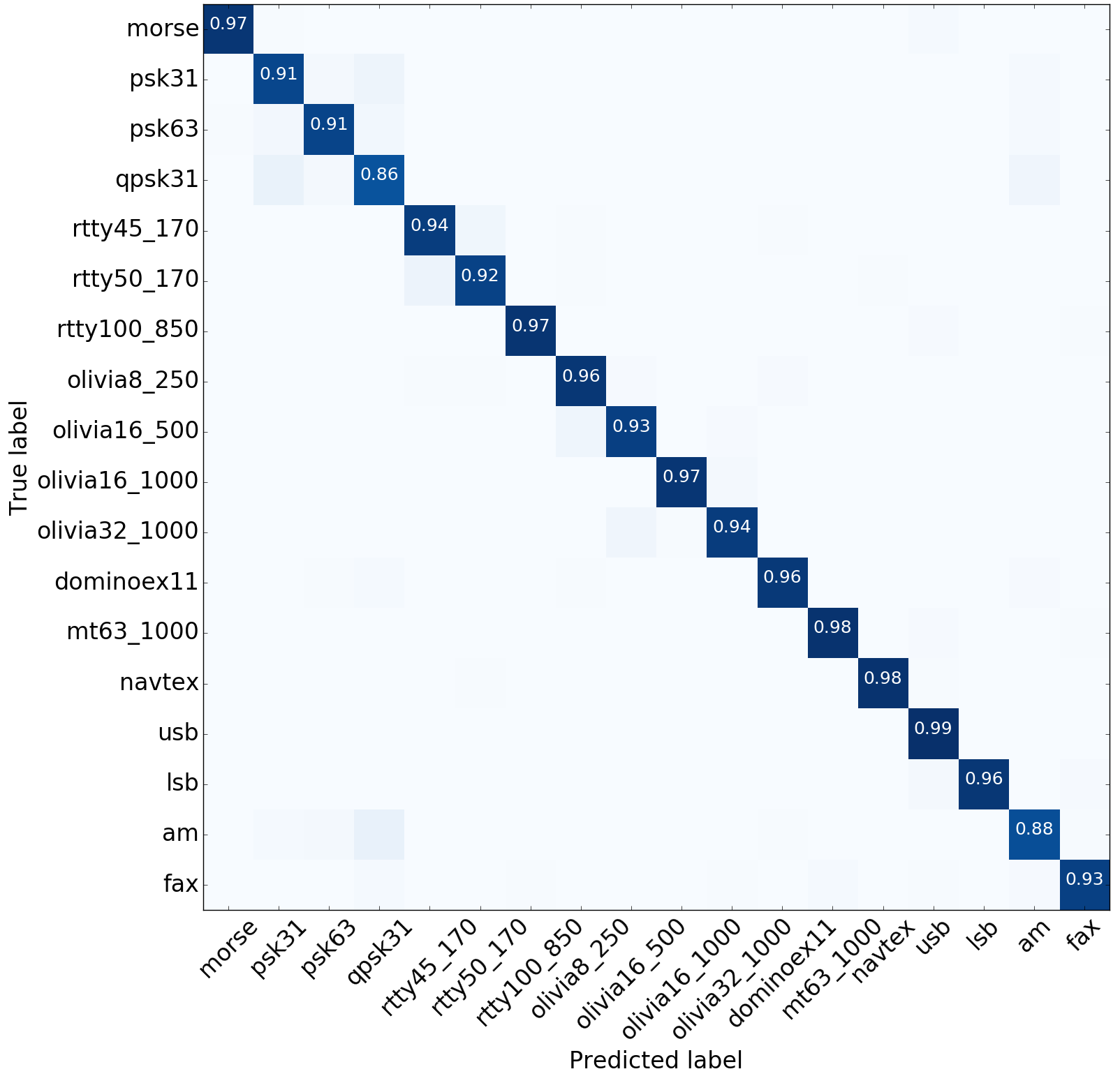
The confusion matrix for the residual net is shown below. Since the overall performance of the net is very good, confusions are very rare. Minor confusions occur between QPSK and BPSK modes. Also RTTY45 and RTTY50 tend to be confused in rare cases, because the only difference between these modes is the slightly deviating baud rate of 45 and 50. Although LSB and USB are quite similar modes, they are classified with very high reliability.